The Data Science Lab
Ordinal Classification Using PyTorch
Dr. James McCaffrey of Microsoft Research presents a simple technique he has used with good success, previously unpublished and without a standard name.
The goal of an ordinal classification problem is to predict a discrete value, where the set of possible values is ordered. For example, you might want to predict the price of a house (based on predictors such as area, number of bedrooms and so on) where the possible price values are 0 (low), 1 (medium), 2 (high), 3 (very high). Ordinal classification is different from a standard, non-ordinal classification problem where the set of values to predict is categorical and is not ordered. For example, predicting the exterior color of a car, where 0 = white,1 = silver, 2 = black and so on is a standard classification problem.
There are a surprisingly large number of techniques for ordinal classification. This article presents a relatively simple technique that I've used with good success. To the best of my knowledge the technique has not been published and does not have a standard name. Briefly, the idea is to programmatically convert ordinal labels such as (0, 1, 2, 3) to floating point targets such as (0.125, 0.375, 0.625, 0.875) and then use a neural network regression approach.
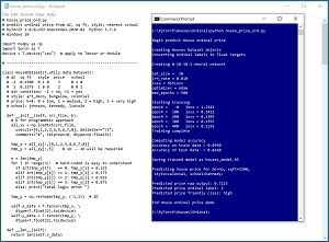
A good way to see where this article is headed is to take a look at the screenshot of a demo program in Figure 1. The demo predicts the price of a house (0 = low, 1 = medium, 2 = high, 3 = very high) based on predictor variables (air conditioning, -1 = no, +1 = yes), normalized area in square feet (e.g., 0.2500 = 2,500 sq. feet), style (art_deco, bungalow, colonial) and local school (johnson, kennedy, lincoln).
The demo loads a 200-item set of training data, and a 40-item set of test data into memory. During the loading process, the ordinal class labels (0, 1, 2, 3) are converting to float targets (0.125, 0.375, 0.625, 0.875). The mapping of ordinal labels to float targets will be explained shortly.
The demo creates an 8-(10-10)-1 deep neural network. There are 8 input nodes (one for each predictor value after encoding house style and local school), two hidden layers with 10 processing nodes each and a single output node. The neural network emits an output value in the range 0.0 to 1.0, that corresponds to the float targets.
After training, the model achieves a prediction accuracy of 89.5 percent on the training data (179 of 200 correct) and 82.5 percent accuracy on the test data (33 of 40 correct). The demo concludes by making a prediction for a new, previously unseen house. The predictor values are air conditioning = no (-1), area = 0.2300 (2300 square feet), style = colonial (0, 0, 1) and local school = kennedy (0, 1, 0). The raw computed output value is 0.7215 which maps to class label 2, which corresponds to an ordinal price of "high."
 [Click on image for larger view.] Figure 1: Ordinal Classification in Action
This article assumes you have an intermediate or better familiarity with PyTorch regression. If necessary, you can get up to speed by reviewing the four-part series "Neural Regression Using PyTorch."
To run the demo program, you must have Python and PyTorch installed on your machine. The demo programs were developed on Windows 10 using the Anaconda 2020.02 64-bit distribution (which contains Python 3.7.6) and PyTorch version 1.8.0 for CPU installed via pip. You can find detailed step-by-step installation instructions for this configuration in my blog post.
The complete demo program source code is presented in this article, and the code is also available in the accompanying file download. The training and test data are embedded as comments at the bottom of the source code.
The Houses Data
The Houses data is synthetic and was generated programmatically. There are a total of 240 data items, divided into a 200-item training dataset and a 40-item test dataset. The raw data looks like:
-1   0.3175   1   0   0   3   0   1   0
 1   0.1975   0   1   0   2   0   0   1
-1   0.1275   0   1   0   0   0   0   1
. . .
Each line of tab-delimited data represents a house. The first value is air conditioning (-1 = no, +1 = yes). The second value is the house area in square feet, normalized by dividing by 10,000. The third through fifth values are house style, one-hot encoded as art_deco = (1, 0, 0), bungalow = (0, 1, 0), colonial = (0, 0, 1). The sixth value is the ordinal price to predict, 0 = low, 1 = medium, 2 = high, 3 = very high. The seventh through ninth values are the local school for the house, one-hot encoded as johnson = (1, 0, 0), kennedy = (0, 1, 0), lincoln = (0, 0, 1).
It's not always easy to determine if a variable to predict is ordinal or not. One rule of thumb is to ask yourself if it makes sense to say one value "is greater than" another. For a house price, it does makes sense to say a medium price (class 1) is greater than a low price (class 0). But for a car color, it doesn't make sense to say that, "Red (color 3) is greater than Blue (color 1)." However, suppose the variable to predict is a person's political leaning, 0 = conservative, 1 = moderate, 2 = liberal. Such data could be considered ordinal (where political learning is a continuum from less liberal to more liberal) or the data could be considered categorical.
Mapping Ordinal Labels to Float Targets
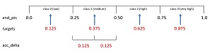
The key to the ordinal classification technique presented in this article is mapping a set of ordinal class labels to a set of floating point targets. The technique is best explained using a concrete example. Suppose there are k = 4 ordinal labels, (0, 1, 2, 3), as in the house data. The four corresponding floating point target values are (0.125, 0.375, 0.625, 0.875). See Figure 2.
 [Click on image for larger view.] Figure 2: Mapping Ordinal Labels to Floating Point Targets
For k = 4, there are four intervals on the unit line from 0.0 to 1.0 so each interval is 1 / k = 0.25 wide. The floating point target values are the midpoints of each interval so the first float target is (1 / k) / 2 = 0.125. Each succeeding target is the value of the previous target plus the interval width of 0.25, so the second float target is first target + 0.25 = 0.375 and so on.
In order to compute prediction accuracy, you compare a computed output value, such as 0.333 with the known target value from the training data, such as 0.375. If the computed output value is within an accuracy delta of 0.125 compared to the target value, the prediction is correct, otherwise the prediction is wrong. For a given k, the accuracy delta is the same as midpoint of the first class interval.
Instead of k = 4 classes as in the demo, suppose there are k = 5 classes. Each interval would be 1 / k = 0.20 wide. The first float target would be 0.20 / 2 = 0.10. The five float targets would be (0.10, 0.30, 0.50, 0.70, 0.90). The accuracy delta would be 0.10.
When making a prediction, in most cases you'll want to map a computed output value, such as 0.667, to the corresponding class label (2 for k = 4 as in the demo). To do so, you determine the interval end points (0.0, 0.25, 0.50, 0.75, 1.0) and then compute which interval the computed output value lies within.
The Complete Demo Program
The complete demo program is presented in Listing 1. All the control logic is contained in program-defined main() and train() functions. The program begins with:
import numpy as np
import torch as T
device = T.device("cpu")

def main():
  # 0. get started
  print("Begin predict House ordinal price ")
  T.manual_seed(1)
  np.random.seed(1)
. . .
In general it's a good idea to set the NumPy and PyTorch global random number seeds to try and get reproducible results, even though for technical reasons this isn't always possible. The seed values of 1 were used only because they gave representative results.
Listing 1: Complete Ordinal Classification Program and Data
# house_price_ord.py
# predict ordinal price from AC, sq ft, style, nearest school
# PyTorch 1.8.0-CPU Anaconda3-2020.02 Python 3.7.6
# Windows 10
import numpy as np
import torch as T
device = T.device("cpu") # apply to Tensor or Module
# -----------------------------------------------------------
class HouseDataset(T.utils.data.Dataset):
# AC sq ft style price school
# -1 0.2500 0 1 0 3 0 1 0
# 1 0.1275 1 0 0 2 0 0 1
# air condition: -1 = no, +1 = yes
# style: art_deco, bungalow, colonial
# price: k=4: 0 = low, 1 = medium, 2 = high, 3 = very high
# school: johnson, kennedy, lincoln
def __init__(self, src_file, k):
# k for programmtic approach
all_xy = np.loadtxt(src_file,
usecols=[0,1,2,3,4,5,6,7,8], delimiter="\t",
comments="#", skiprows=0, dtype=np.float32)
tmp_x = all_xy[:,[0,1,2,3,4,6,7,8]]
tmp_y = all_xy[:,5] # 1D -- 2D will be required
n = len(tmp_y)
for i in range(n): # hard-coded is easy to understand
if int(tmp_y[i]) == 0: tmp_y[i] = 0.125
elif int(tmp_y[i]) == 1: tmp_y[i] = 0.375
elif int(tmp_y[i]) == 2: tmp_y[i] = 0.625
elif int(tmp_y[i]) == 3: tmp_y[i] = 0.875
else: print("Fatal logic error ")
tmp_y = np.reshape(tmp_y, (-1,1)) # 2D
self.x_data = T.tensor(tmp_x, \
dtype=T.float32).to(device)
self.y_data = T.tensor(tmp_y, \
dtype=T.float32).to(device)
def __len__(self):
return len(self.x_data)
def __getitem__(self, idx):
preds = self.x_data[idx,:] # or just [idx]
price = self.y_data[idx,:]
return (preds, price) # tuple of two matrices
# -----------------------------------------------------------
class Net(T.nn.Module):
def __init__(self):
super(Net, self).__init__()
self.hid1 = T.nn.Linear(8, 10) # 8-(10-10)-1
self.hid2 = T.nn.Linear(10, 10)
self.oupt = T.nn.Linear(10, 1) # [0.0 to 1.0]
T.nn.init.xavier_uniform_(self.hid1.weight)
T.nn.init.zeros_(self.hid1.bias)
T.nn.init.xavier_uniform_(self.hid2.weight)
T.nn.init.zeros_(self.hid2.bias)
T.nn.init.xavier_uniform_(self.oupt.weight)
T.nn.init.zeros_(self.oupt.bias)
def forward(self, x):
z = T.tanh(self.hid1(x))
z = T.tanh(self.hid2(z))
z = T.sigmoid(self.oupt(z)) #
return z
# -----------------------------------------------------------
def accuracy(model, ds, k):
n_correct = 0; n_wrong = 0
acc_delta = (1.0 / k) / 2 # if k=4 delta = 0.125
for i in range(len(ds)): # each input
(X, y) = ds[i] # (predictors, target)
with T.no_grad(): # y target is like 0.375
oupt = model(X) # oupt is in [0.0, 1.0]
if T.abs(oupt - y) < = acc_delta:
n_correct += 1
else:
n_wrong += 1
acc = (n_correct * 1.0) / (n_correct + n_wrong)
return acc
# -----------------------------------------------------------
def train(net, ds, bs, lr, me, le):
# network, dataset, batch_size, learn_rate,
# max_epochs, log_every
train_ldr = T.utils.data.DataLoader(ds,
batch_size=bs, shuffle=True)
loss_func = T.nn.MSELoss()
opt = T.optim.Adam(net.parameters(), lr=lr)
for epoch in range(0, me):
# T.manual_seed(1+epoch) # recovery reproducibility
epoch_loss = 0 # for one full epoch
for (b_idx, batch) in enumerate(train_ldr):
(X, y) = batch # (predictors, targets)
opt.zero_grad() # prepare gradients
oupt = net(X) # predicted prices
loss_val = loss_func(oupt, y) # a tensor
epoch_loss += loss_val.item() # accumulate
loss_val.backward() # compute gradients
opt.step() # update weights
if epoch % le == 0:
print("epoch = %4d loss = %0.4f" % \
(epoch, epoch_loss))
# TODO: save checkpoint
# -----------------------------------------------------------
def float_oupt_to_class(oupt, k):
end_pts = np.zeros(k+1, dtype=np.float32)
delta = 1.0 / k
for i in range(k):
end_pts[i] = i * delta
end_pts[k] = 1.0
# if k=4, [0.0, 0.25, 0.50, 0.75, 1.0]
for i in range(k):
if oupt >= end_pts[i] and oupt <= end_pts[i+1]:
return i
return -1 # fatal error
# -----------------------------------------------------------
def main():
# 0. get started
print("\nBegin predict House ordinal price \n")
T.manual_seed(1) # representative results
np.random.seed(1)
# 1. create Dataset objects
print("Creating Houses Dataset objects ")
print("Converting ordinal labels to float targets ")
train_file = ".\\Data\\houses_train_ord.txt"
train_ds = HouseDataset(train_file, k=4) # 200 rows
test_file = ".\\Data\\houses_test_ord.txt"
test_ds = HouseDataset(test_file, k=4) # 40 rows
# 2. create network
print("\nCreating 8-10-10-1 neural network ")
net = Net().to(device)
net.train() # set mode
# 3. train model
bat_size = 10
lrn_rate = 0.010
max_epochs = 500
log_every = 100
print("\nbat_size = %3d " % bat_size)
print("lrn_rate = %0.3f " % lrn_rate)
print("loss = MSELoss ")
print("optimizer = Adam ")
print("max_epochs = %3d " % max_epochs)
print("\nStarting training ")
train(net, train_ds, bat_size, lrn_rate,
max_epochs, log_every)
print("Training complete ")
# 4. evaluate model accuracy
print("\nComputing model accuracy")
net.eval() # set mode
acc_train = accuracy(net, train_ds, k=4)
print("Accuracy on train data = %0.4f" % \
acc_train)
acc_test = accuracy(net, test_ds, k=4)
print("Accuracy on test data = %0.4f" % \
acc_test)
# 5. save trained model (TODO)
print("\nSaving trained model as houses_model.h5 ")
# model.save_weights(".\\Models\\houses_model_wts.h5")
# model.save(".\\Models\\houses_model.h5")
# 6. make a prediction
print("\nPredicting house price for AC=no, sqft=2300, ")
print(" style=colonial, school=kennedy: ")
unk = np.array([[-1, 0.2300, 0,0,1, 0,1,0]],
dtype=np.float32)
unk = T.tensor(unk, dtype=T.float32).to(device)
with T.no_grad():
pred_price = net(unk)
pred_price = pred_price.item() # scalar 0.0 to 1.0
print("\nPredicted price raw output: %0.4f" % \
pred_price)
labels = ["low", "medium", "high", "very high"]
c = float_oupt_to_class(pred_price, k=4)
print("Predicted price ordinal label: %d " % c)
print("Predicted price friendly class: %s " % \
labels[c])
print("\nEnd House ordinal price demo")
if __name__ == "__main__":
main()
# ===========
# houses_train_ord.txt
# AC (-1 = no), sq_ft, style (one-hot)
# price (0=low, 1=med, 2=high, 3=v. high),
# school (one-hot)
# -1 0.1275 0 1 0 0 0 0 1
# 1 0.1100 1 0 0 0 1 0 0
# -1 0.1375 0 0 1 0 0 1 0
# 1 0.1975 0 1 0 2 0 0 1
# -1 0.1200 0 0 1 0 1 0 0
# -1 0.2500 0 1 0 2 0 1 0
# 1 0.1275 1 0 0 1 0 0 1
# -1 0.1750 0 0 1 1 0 0 1
# -1 0.2500 0 1 0 2 0 0 1
# 1 0.1800 0 1 0 1 1 0 0
# 1 0.0975 1 0 0 0 0 0 1
# -1 0.1100 0 1 0 0 0 1 0
# 1 0.1975 0 0 1 1 0 0 1
# -1 0.3175 1 0 0 3 0 1 0
# -1 0.1700 0 1 0 1 1 0 0
# 1 0.1650 0 1 0 1 0 1 0
# -1 0.2250 0 1 0 2 0 1 0
# -1 0.2125 0 1 0 2 0 1 0
# 1 0.1675 0 1 0 1 0 1 0
# 1 0.1550 1 0 0 1 0 1 0
# -1 0.1375 0 0 1 0 1 0 0
# -1 0.2425 0 1 0 2 1 0 0
# 1 0.3200 0 0 1 3 0 1 0
# -1 0.3075 1 0 0 3 0 1 0
# -1 0.2700 1 0 0 2 0 0 1
# 1 0.1700 0 1 0 1 0 0 1
# -1 0.1475 1 0 0 1 1 0 0
# -1 0.2500 0 1 0 2 0 0 1
# -1 0.2750 1 0 0 2 0 0 1
# -1 0.2000 1 0 0 2 1 0 0
# -1 0.1100 0 0 1 0 1 0 0
# -1 0.3400 1 0 0 3 0 1 0
# 1 0.3000 0 0 1 3 1 0 0
# 1 0.1550 0 1 0 1 0 1 0
# -1 0.2150 0 1 0 1 0 0 1
# -1 0.2900 0 0 1 3 0 1 0
# 1 0.2750 0 0 1 2 0 1 0
# 1 0.2175 0 1 0 2 0 1 0
# 1 0.2150 0 1 0 2 0 0 1
# 1 0.1050 1 0 0 1 1 0 0
# -1 0.2775 1 0 0 2 0 0 1
# -1 0.3225 1 0 0 3 0 1 0
# 1 0.2075 0 1 0 2 1 0 0
# -1 0.3225 1 0 0 3 0 0 1
# 1 0.2800 0 0 1 3 0 0 1
# -1 0.1575 0 1 0 1 0 0 1
# 1 0.3250 0 0 1 3 0 0 1
# -1 0.2750 1 0 0 2 0 0 1
# 1 0.1250 1 0 0 1 1 0 0
# -1 0.2325 0 1 0 2 0 0 1
# 1 0.1825 1 0 0 2 1 0 0
# -1 0.2600 0 1 0 2 0 1 0
# -1 0.3075 1 0 0 3 0 0 1
# -1 0.2875 1 0 0 3 0 0 1
# 1 0.2300 0 1 0 2 0 1 0
# 1 0.3100 0 0 1 3 1 0 0
# -1 0.2750 1 0 0 2 0 0 1
# 1 0.1125 0 1 0 0 0 0 1
# 1 0.2525 1 0 0 2 1 0 0
# 1 0.1625 0 1 0 1 0 1 0
# 1 0.1075 1 0 0 1 0 0 1
# -1 0.2200 0 1 0 2 0 1 0
# -1 0.2300 0 1 0 2 0 1 0
# -1 0.3100 1 0 0 3 0 1 0
# -1 0.2875 1 0 0 3 0 1 0
# 1 0.3375 0 0 1 3 0 0 1
# -1 0.1450 0 0 1 0 1 0 0
# -1 0.2650 1 0 0 2 1 0 0
# 1 0.2225 0 1 0 2 1 0 0
# -1 0.2300 0 1 0 2 0 1 0
# 1 0.1025 0 1 0 0 0 1 0
# 1 0.1925 0 1 0 2 1 0 0
# -1 0.2525 0 1 0 2 0 1 0
# -1 0.1650 0 1 0 1 0 1 0
# 1 0.1650 0 1 0 1 0 1 0
# -1 0.1300 1 0 0 1 0 1 0
# -1 0.2900 1 0 0 3 1 0 0
# -1 0.2175 0 1 0 1 0 0 1
# 1 0.2300 1 0 0 2 1 0 0
# -1 0.3000 1 0 0 3 1 0 0
# 1 0.2125 0 1 0 1 1 0 0
# 1 0.2825 0 0 1 2 0 0 1
# 1 0.3125 0 0 1 3 0 1 0
# 1 0.2500 0 1 0 2 1 0 0
# -1 0.2375 0 1 0 2 0 0 1
# 1 0.3375 0 0 1 3 0 1 0
# 1 0.2000 0 1 0 2 0 0 1
# -1 0.2100 0 1 0 1 0 1 0
# -1 0.3225 1 0 0 3 1 0 0
# 1 0.2375 0 0 1 2 1 0 0
# -1 0.2250 0 1 0 2 0 1 0
# 1 0.1250 1 0 0 1 0 0 1
# -1 0.1925 1 0 0 1 1 0 0
# -1 0.2750 0 1 0 2 0 0 1
# 1 0.2200 0 1 0 2 1 0 0
# -1 0.1675 0 1 0 1 1 0 0
# -1 0.1700 0 1 0 1 0 0 1
# -1 0.1350 0 0 1 0 0 1 0
# -1 0.1600 0 1 0 1 0 1 0
# -1 0.2125 0 1 0 1 0 0 1
# 1 0.1200 1 0 0 1 0 0 1
# -1 0.2100 0 1 0 2 0 1 0
# -1 0.1250 0 0 1 0 0 0 1
# -1 0.2550 0 1 0 2 0 1 0
# 1 0.2750 0 0 1 2 0 1 0
# -1 0.2200 0 0 1 1 1 0 0
# 1 0.0925 1 0 0 1 1 0 0
# 1 0.3350 0 0 1 3 0 1 0
# -1 0.2250 0 1 0 2 0 0 1
# -1 0.2425 0 1 0 2 1 0 0
# 1 0.1275 0 1 0 1 0 1 0
# 1 0.3350 0 1 0 3 1 0 0
# -1 0.1850 0 1 0 1 0 0 1
# 1 0.1600 0 1 0 1 1 0 0
# -1 0.2400 0 1 0 2 1 0 0
# 1 0.3300 0 0 1 3 0 0 1
# -1 0.3075 1 0 0 3 1 0 0
# 1 0.2900 0 1 0 3 0 0 1
# -1 0.0950 0 0 1 0 1 0 0
# -1 0.1900 0 1 0 1 0 0 1
# 1 0.1375 0 1 0 1 1 0 0
# -1 0.2100 0 1 0 1 1 0 0
# -1 0.3025 1 0 0 3 1 0 0
# 1 0.1375 1 0 0 0 0 0 1
# -1 0.1475 1 0 0 1 0 1 0
# 1 0.2150 0 1 0 2 1 0 0
# -1 0.2400 0 1 0 2 1 0 0
# -1 0.1375 0 0 1 0 0 0 1
# 1 0.2200 1 0 0 2 1 0 0
# -1 0.1150 0 0 1 0 0 1 0
# 1 0.1825 0 0 1 2 0 1 0
# -1 0.3225 1 0 0 3 0 0 1
# -1 0.1450 0 0 1 0 0 0 1
# 1 0.1675 0 1 0 1 1 0 0
# 1 0.3325 0 0 1 3 0 1 0
# 1 0.1075 1 0 0 0 0 0 1
# -1 0.1350 0 0 1 0 1 0 0
# -1 0.1450 0 0 1 0 1 0 0
# 1 0.1575 0 1 0 1 1 0 0
# -1 0.1825 0 1 0 1 0 0 1
# -1 0.2450 0 1 0 2 0 1 0
# 1 0.1425 1 0 0 1 1 0 0
# 1 0.2175 0 1 0 2 0 0 1
# 1 0.2325 0 1 0 2 0 1 0
# -1 0.2875 1 0 0 3 1 0 0
# 1 0.2625 0 1 0 2 0 0 1
# 1 0.1575 0 1 0 1 0 0 1
# 1 0.2750 0 0 1 2 1 0 0
# -1 0.2500 0 1 0 2 1 0 0
# -1 0.2400 0 1 0 2 0 1 0
# 1 0.1100 1 0 0 0 0 0 1
# -1 0.2975 1 0 0 3 0 0 1
# -1 0.1725 0 0 1 1 1 0 0
# 1 0.3225 0 0 1 3 1 0 0
# -1 0.1450 0 0 1 0 0 0 1
# 1 0.1725 0 1 0 1 0 1 0
# 1 0.3050 0 0 1 3 1 0 0
# -1 0.3200 1 0 0 3 0 0 1
# 1 0.1450 1 0 0 1 1 0 0
# -1 0.3175 1 0 0 3 0 1 0
# 1 0.1475 1 0 0 1 0 1 0
# 1 0.2575 0 1 0 2 1 0 0
# 1 0.1200 1 0 0 1 0 0 1
# -1 0.2425 0 1 0 2 0 1 0
# -1 0.0900 1 0 0 0 1 0 0
# -1 0.0925 0 0 1 0 1 0 0
# -1 0.1650 0 0 1 1 0 1 0
# 1 0.1025 1 0 0 0 0 0 1
# -1 0.1475 0 0 1 0 0 0 1
# 1 0.2225 1 0 0 2 0 0 1
# 1 0.3250 1 0 0 3 0 0 1
# 1 0.2800 0 0 1 2 1 0 0
# 1 0.2625 0 1 0 2 0 0 1
# 1 0.1450 1 0 0 1 0 1 0
# 1 0.2350 0 1 0 2 0 1 0
# -1 0.3425 0 0 1 3 1 0 0
# -1 0.1575 0 1 0 1 0 0 1
# -1 0.3075 0 0 1 2 0 1 0
# -1 0.0950 0 0 1 0 0 1 0
# -1 0.1925 0 1 0 1 0 0 1
# 1 0.1300 1 0 0 1 1 0 0
# -1 0.3075 1 0 0 3 0 1 0
# -1 0.2000 0 1 0 1 1 0 0
# 1 0.2475 0 1 0 3 1 0 0
# -1 0.2825 1 0 0 3 1 0 0
# 1 0.2425 0 1 0 3 0 1 0
# -1 0.2625 0 0 1 2 1 0 0
# 1 0.0900 1 0 0 0 1 0 0
# 1 0.2800 0 0 1 2 0 0 1
# 1 0.2600 0 1 0 2 0 1 0
# 1 0.0900 0 1 0 0 0 1 0
# 1 0.2900 0 0 1 3 1 0 0
# 1 0.1950 0 1 0 2 0 1 0
# 1 0.2325 0 1 0 2 1 0 0
# 1 0.2025 0 1 0 1 0 1 0
# 1 0.3025 0 0 1 3 1 0 0
# -1 0.1800 0 0 1 1 0 1 0
# -1 0.2225 0 1 0 2 1 0 0
# -1 0.1425 0 0 1 0 1 0 0
# -1 0.2725 1 0 0 2 0 0 1
#
# houses_test_ord.txt
# 1 0.2550 0 1 0 2 1 0 0
# 1 0.1625 0 1 0 1 0 1 0
# -1 0.2750 1 0 0 2 1 0 0
# -1 0.1275 0 0 1 0 0 0 1
# -1 0.1650 0 0 1 1 0 0 1
# 1 0.1450 1 0 0 1 0 1 0
# -1 0.3275 1 0 0 3 1 0 0
# 1 0.2175 0 1 0 2 0 1 0
# 1 0.2725 0 0 1 2 0 1 0
# -1 0.3075 1 0 0 3 0 1 0
# -1 0.2600 1 0 0 2 0 1 0
# -1 0.1525 0 0 1 0 0 1 0
# -1 0.1450 0 0 1 0 1 0 0
# 1 0.2375 0 1 0 2 0 0 1
# -1 0.1950 0 1 0 1 0 1 0
# -1 0.2375 0 1 0 2 0 0 1
# 1 0.2475 0 1 0 2 1 0 0
# 1 0.3150 0 0 1 3 0 0 1
# 1 0.1525 1 0 0 1 1 0 0
# 1 0.3050 0 0 1 3 0 0 1
# 1 0.2350 0 1 0 2 0 0 1
# -1 0.1525 0 0 1 0 0 0 1
# 1 0.2550 0 1 0 2 0 0 1
# 1 0.1200 0 1 0 1 1 0 0
# 1 0.2450 0 1 0 2 1 0 0
# -1 0.3300 1 0 0 3 0 0 1
# 1 0.3275 1 0 0 3 1 0 0
# 1 0.2300 1 0 0 2 0 1 0
# 1 0.2275 0 1 0 2 0 0 1
# 1 0.2350 1 0 0 2 1 0 0
# 1 0.1475 1 0 0 1 1 0 0
# 1 0.2850 0 0 1 3 0 0 1
# 1 0.1000 0 0 1 0 1 0 0
# 1 0.1750 0 1 0 1 1 0 0
# 1 0.3075 0 0 1 3 0 0 1
# 1 0.1550 0 1 0 1 0 0 1
# -1 0.0925 0 0 1 0 1 0 0
# -1 0.1300 0 0 1 0 0 0 1
# 1 0.1425 0 0 1 1 1 0 0
# 1 0.2975 0 0 1 3 0 0 1
Next, the demo loads the training and test data into memory:
  # 1. create Dataset objects
  print("Creating Houses Dataset objects ")
  print("Converting ordinal labels to float targets ")
  train_file = ".\\Data\\houses_train_ord.txt"
  train_ds = HouseDataset(train_file, k=4)  # 200 rows

  test_file = ".\\Data\\houses_test_ord.txt"
  test_ds = HouseDataset(test_file, k=4)  # 40 rows
The HouseDataset object is derived from the PyTorch Dataset class. Data is loaded into memory, and the ordinals class labels are programmatically converted to floating point target values using the scheme described in the previous section. The conversion from ordinal label to float target is hard-coded:
    n = len(tmp_y)
    for i in range(n):
      if int(tmp_y[i])   == 0: tmp_y[i] = 0.125
      elif int(tmp_y[i]) == 1: tmp_y[i] = 0.375
      elif int(tmp_y[i]) == 2: tmp_y[i] = 0.625
      elif int(tmp_y[i]) == 3: tmp_y[i] = 0.875
      else: print("Fatal logic error ")
In my opinion, using a hard-coded conversion approach is simpler and easier to understand than using a programmatic approach.
After the training and test data is loaded, the demo creates an 8-(10-10)-1 neural network regression system:
  # 2. create network
  print("Creating 8-10-10-1 neural network ")
  net = Net().to(device)
  net.train()   # set training mode
Th number of input nodes is determined by the problem data. There is one output node because the network must emit a single floating point value between 0.0 and 1.0. The number of hidden layers and the number of nodes in each layer are hyperparameters that must be determined by trial and error.
Next, the demo trains the network:
  # 3. train model
  bat_size = 10
  lrn_rate = 0.010
  max_epochs = 500
  log_every = 100
  . . .
  print("Starting training ")
  train(net, train_ds, bat_size, lrn_rate,
    max_epochs, log_every)
  print("Training complete ")
Training the network model is performed by a program-defined train() function which uses a hard-coded Adam optimizer object and hard-coded MSELoss (mean squared error). Adam tends to work a bit better than basic SGD optimization. The batch size (10), learning rate (0.010) and number of training epochs (500) are all hyperparameters.
Next, the demo computes the model accuracy on the training and test data:
  # 4. evaluate model accuracy
  print("Computing model accuracy")
  net.eval()  # set mode
  acc_train = accuracy(net, train_ds, k=4)
  print("Accuracy on train data = %0.4f" % \
    acc_train)
  acc_test = accuracy(net, test_ds, k=4)
  print("Accuracy on test data  = %0.4f" % \
    acc_test)
The accuracy() function is program defined. The function accepts the number of classes as a parameter k, so that the accuracy delta of (1 / k) / 2 can be computed.
At this point, in a non-demo scenario, you'd save your trained model to file. The demo skips this step and finishes up by making a house price prediction for a new, previously unseen house. First, predictor variables are set up:
  # 6. make a prediction
  print("Predicting house price for AC=no, sqft=2300, ")
  print(" style=colonial, school=kennedy: ")
  unk = np.array([[-1, 0.2300,  0,0,1,  0,1,0]],
    dtype=np.float32)
  unk = T.tensor(unk, dtype=T.float32).to(device)
Notice that the predictor values are stored into a 2D NumPy array, indicated by the double square brackets, rather than a 1D array. This is one of the many small syntax issues that make learning PyTorch (or TensorFlow or Keras) very difficult.
Next, the demo feeds the input values to the trained model:
  with T.no_grad():
    pred_price = net(unk)
  pred_price = pred_price.item()  # scalar in 0.0 to 1.0
  print("Predicted price raw output: %0.4f" % pred_price)
The no_grad() statement is used so that the computed output value doesn't become part of the internal network computational graph. The item() method is used to extract the single value in the output Tensor object and convert it to a NumPy numeric value. One of the points here is that when working with neural systems, even seemingly simple operations can have subtle factors.
The demo concludes by converting the raw computed output to a more human-friendly form:
. . .
  labels = ["low", "medium", "high", "very high"]
  c = float_oupt_to_class(pred_price, k=4)
  print("Predicted price ordinal label: %d " % c)
  print("Predicted price friendly class: %s " % labels[c])
  print("End House ordinal price demo")
if __name__ == "__main__":
  main()
Program-defined function float_oupt_to_class() converts the raw output (0.7215) to the associated class label (2) using the mini-algorithm in the section that explains label-to-float target mapping.
Wrapping Up
When working with an ordinal classification problem, it's possible to ignore the ordering attribute of the class labels and just use standard multi-class classification. But this approach doesn't use all available information. For example, suppose k = 5 and the class labels correspond to ratings of (0 = bad, 1 = weak, 2 = average, 3 = good, 4 = excellent). And suppose a target label for an item in the training data is 4 = excellent. Using standard multi-class classification, a predicted output of 0 = bad has the same error as a predicted output of 3 = good. The ordinal classification technique presented in this article would assign greater error to 0 = bad.