The Data Science Lab
Quadratic Regression with SGD Training Using JavaScript
Dr. James McCaffrey presents a complete end-to-end demonstration of quadratic regression, with SGD training, implemented from scratch, using JavaScript. Compared to standard linear regression, quadratic regression is better able to handle data with a non-linear structure, and data with interactions between predictor variables.
The goal of a machine learning regression problem is to predict a single numeric value. For example, you might want to predict an employee's salary based on age, IQ test score, high school grade point average, and so on. There are approximately a dozen common regression techniques. The most basic technique is called linear regression, or sometimes multiple linear regression, where the "multiple" indicates two or more predictor variables.
The form of a basic linear regression prediction model is y' = (w0 * x0) + (w1 * x1) + . . + b, where y' is the predicted value, the xi are predictor values, the wi are weights, and b is the bias. Quadratic regression extends linear regression. The form of a quadratic regression model is y' = (w0 * x0) + . . + (wn * xn) + (wj * x0 * x0) + . . + (wk * x0 * x1) + . . . + b. There are derived predictors that are the square of each original predictor, and interaction terms that are the multiplication product of all possible pairs of original predictors.
Compared to basic linear regression, quadratic regression can handle more complex data. And compared to the most powerful regression techniques that are designed to handle complex data, quadratic regression often has slightly worse prediction accuracy, but is much easier to implement and train, and has much better model interpretability.
This article presents a demo of quadratic regression, implemented from scratch, trained with stochastic gradient descent (SGD), using the JavaScript language. A good way to see where this article is headed is to take a look at the screenshot in Figure 1. The demo program begins by loading synthetic training and test data into memory. The data looks like:
-0.1660, 0.4406, -0.9998, -0.3953, -0.7065, 0.4840
 0.0776, -0.1616, 0.3704, -0.5911, 0.7562, 0.1568
-0.9452, 0.3409, -0.1654, 0.1174, -0.7192, 0.8054
 0.9365, -0.3732, 0.3846, 0.7528, 0.7892, 0.1345
. . .
The first five values on each line are the x predictors. The last value on each line is the target y variable to predict. There are 200 training items and 40 test items.
The demo creates and trains a quadratic regression model, evaluates the model accuracy on the training and test data, and then uses the model to predict the target y value for the first training item x = [-0.1660, 0.4406, -0.9998, -0.3953, -0.7065].
After loading the data from file and displaying the first three training X predictors and training y targets, the demo shows how a quadratic regression model is created and trained:
Creating quadratic regression model
Setting lrnRate = 0.001
Setting maxEpochs = 1000
Starting SGD training
epoch = 0 MSE = 0.0925 acc = 0.0100
epoch = 200 MSE = 0.0003 acc = 0.9050
epoch = 400 MSE = 0.0003 acc = 0.8850
epoch = 600 MSE = 0.0003 acc = 0.8850
epoch = 800 MSE = 0.0003 acc = 0.8850
Done
There are several ways to train a quadratic regression model, including stochastic gradient descent (SGD), pseudo-inverse training, closed form inverse training, L-BFGS optimization training and so on. The demo program uses SGD training, which is iterative and requires a learning rate and a maximum number of epochs. These two parameter values must be determined by trial and error.
The next part of the demo output shows the trained model weights and the bias:
Model base weights:
 -0.2630 0.0354 -0.0420 0.0341 -0.1124

Model quadratic weights:
 0.0655 0.0194 0.0051 0.0047 0.0243

Model interaction weights:
 0.0043 0.0249 0.0071 0.1081 -0.0012 -0.0093
 0.0362 0.0085 -0.0568 0.0016

Model bias: 0.3220
Because the demo data has 5 predictor variables, there are 5 base weights, 5 quadratic (squared term) weights, and (5 * 4) / 2 = 10 interaction weights.
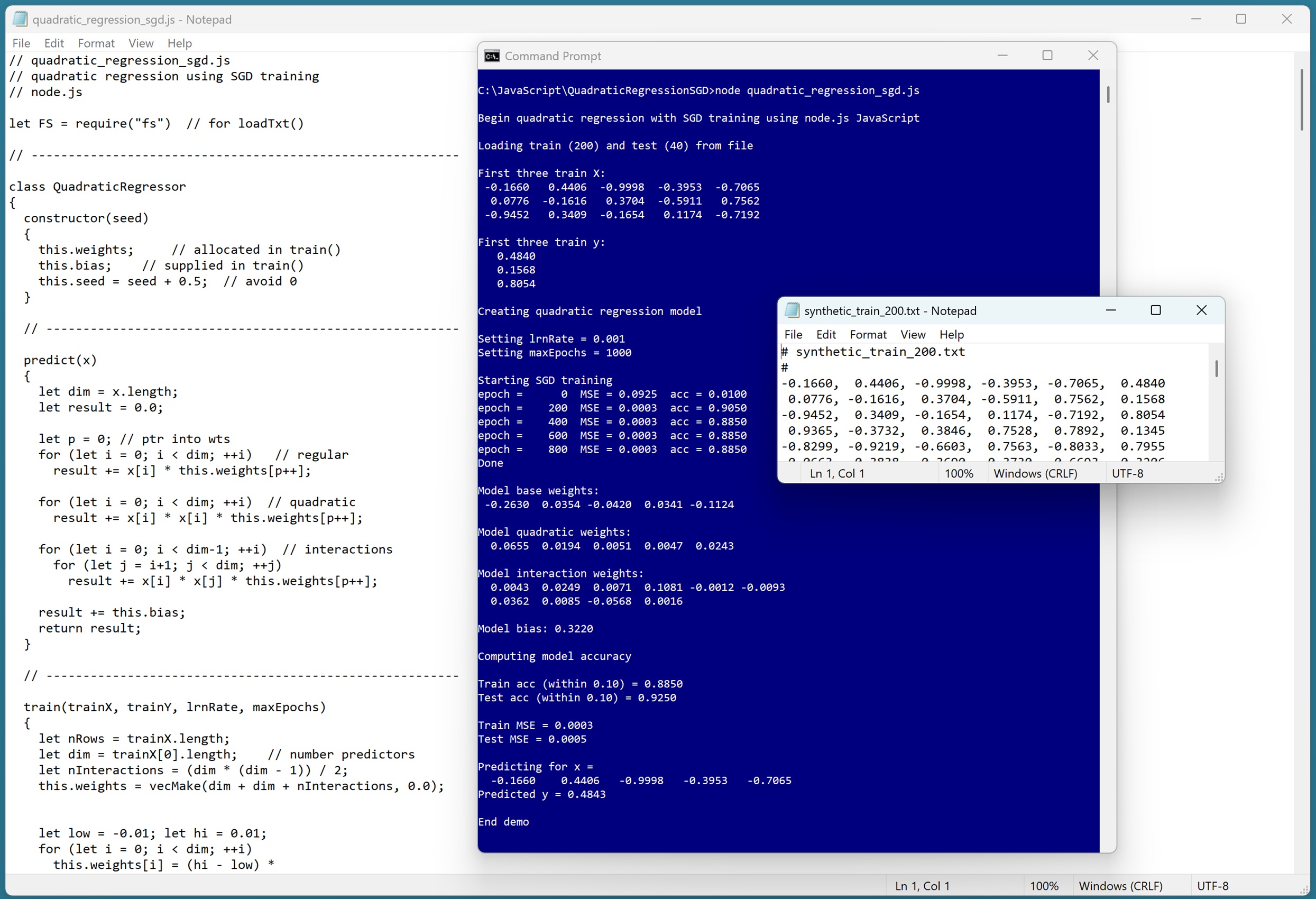 [Click on image for larger view.] Figure 1: Quadratic Regression with SGD Training Using JavaScript in Action.
The demo concludes by evaluating the trained model and making a prediction:
Computing model accuracy

Train acc (within 0.10) = 0.8850
Test acc (within 0.10) = 0.9250

Train MSE = 0.0003
Test MSE = 0.0005

Predicting for x =
 -0.1660 0.4406 -0.9998 -0.3953 -0.7065
Predicted y = 0.4843
The model accuracy is quite good compared to many other regression techniques applied to the synthetic data -- 88.50% accuracy on the training data (177 out of 200 correct) and 92.50% accuracy on the test data (37 out of 40 correct). A prediction is scored as correct if it's within 10% of the true target value.
This article assumes you have intermediate or better programming skill but doesn't assume you know anything about quadratic regression. The demo is implemented using JavaScript but you should be able to refactor the demo code to another C-family language if you wish. All normal error checking has been removed to keep the main ideas as clear as possible.
The source code for the demo program is too long to be presented in its entirety in this article. The complete code and data are available in the accompanying file download, and they're also available online.
The Demo Data
The demo data is synthetic. It was generated by a 5-10-1 neural network with random weights and bias values. The idea here is that the synthetic data does have an underlying, but complex, non-linear structure which can be predicted.
All of the predictor values are between -1 and +1. When using quadratic regression, technically, it's not necessary to normalize/scale the training data. But normalized data is easier to train and often leads to a better prediction model, especially if some raw predictor values are very large (such as employee income) and some values are small (such as employee age). Also, using normalized data allows you to interpret the model weights more easily (larger magnitudes mean more effect on the predicted y value).
Quadratic regression is most often used with data that has strictly numeric predictor variables. It is possible to use the technique with categorical data that has an inherent order using equal-interval encoding. For example, a predictor variable rating with possible values (poor, so-so, good) could be encoded as poor = 0.25, so-so = 0.50, good = 0.75.
However, for categorical data without inherent order, such as job with possible values (management, sales, tech), there's no obvious way to encode the values so that when multiplied together you get a meaningful number. That said, I have seen examples where non-ordered categorical predictor values were equal-interval encoded and the resulting prediction model worked quite well. But there are no solid research results that I'm aware of that support this encoding technique for quadratic regression.
Understanding Quadratic Regression
Suppose, as in the demo data, there are five predictors, aka features, (x0, x1, x2, x3, x4). The prediction equation for basic linear regression is:
y' = (w0 * x0) + (w1 * x1) + (w2 * x2) + (w3 * x3) + (w4 * x4) + b
The wi are model weights (aka coefficients), and b is the model bias (aka intercept). The values of the weights and the bias must be determined by training, so that predicted y' values are close to the known, correct y values in a set of training data.
Basic linear regression is simple but it can't predict well for data that has an underlying non-linear structure, and basic linear regression can't deal with data that has hidden interactions between the xi predictors.
The prediction equation for quadratic regression with five predictors is:
y' = (w0 * x0) + (w1 * x1) + (w2 * x2) + (w3 * x3) + (w4 * x4) +

 (w5 * x0*x0) + (w6 * x1*x1) + (w7 * x2*x2) +
 (w8 * x3*x3) + (w9 * x4*x4) +

 (w10 * x0*x1) + (w11 * x0*x2) + (w12 * x0*x3) + (w13 * x0*x4) +
 (w14 * x1*x2) + (w15 * x1*x3) + (w16 * x1*x4) +
 (w17 * x2*x3) + (w18 * x2*x4) +
 (w19 * x3*x4)

 + b
The squared (aka "quadratic") xi^2 terms handle non-linear structure. If there are n predictors, there are also n squared terms. The xi * xj terms between all possible pairs of original predictors handle interactions between predictors. If there are n predictors, there are (n * (n-1)) / 2 interaction terms.
Therefore, in general, if there are n original predictor variables, there are a total of n + n + (n * (n-1))/2 model weights and one bias. Behind the scenes, the derived xi^2 squared terms and the derived xi*xj interaction terms are computed programmatically on-the-fly, as opposed to explicitly creating an augmented dataset.
A quadratic regression model is trained on the implicit derived data. In spite of the multiplication of the base predictors, the model is still a linear model.
Quadratic regression is a subset of polynomial regression. For example, cubic regression includes xi^3 terms, quartic regression includes xi^4, and so on. In practice, it's rare to go beyond quadratic regression, in part because the number of derived predictors increases quickly. For example, for the demo data with just 5 predictors, cubic regression has 55 derived predictor variables, and quartic regression has 125 derived variables.
Quadratic regression is a superset of linear regression with two-way interactions. Linear regression with two-way interactions includes only the derived xi * xj terms, and omits the xi^2 terms.
Quadratic regression can seem a bit strange if you're new to the technique. Suppose you have a predictor x0 = employee-age and a predictor x1 = employee-income. The x0 * x1 term has no physical meaning -- it's just a new math predictor variable that can deal with hidden interactions between age and income.
Training the Quadratic Regression Model
The demo program uses standard stochastic gradient descent (SGD) optimization to train the model. In high-level pseudo-code:
initialize weights and bias to small random values
loop max_epochs times
shuffle the order of training data
loop each training item
get training inputs X
get training target value actual y
compute predicted y using curr weights and bias
for-each weight and the bias
new_wt = old_wt * -1 * lrn_rate * (pred_y -- actual_y) * x
end-for
end-loop
end-loop
The idea is to adjust each weight so that the predicted y gets closer to the actual y. The (pred_y -- actual_y) is a simple measure of how far off the predicted value is and loosely represents a math gradient. If pred_y is larger than actual_y, you want to decrease the associated weight to make the pred_y smaller.
The learning rate is typically a value like 0.01 that lessens the amount of change in the weights so that there are no wild fluctuations. The learning rate must be determined by trial and error. If the learning rate is too large, SGD training might jump past a good weight value. If the learning rate is too small, training might be too slow.
The -1 term controls the direction of the change in the weight being adjusted. If the difference term was (actual_y -- pred_y), the -1 term could be dropped, but it's traditional to use (pred_y -- actual_y). The x term in the update controls the direction of the weight change, depending on the sign of x, and the amount of change in the weight, depending on the magnitude of x.
The order in which the training data is processed is randomized in each epoch (one complete pass through all items). This prevents training from oscillating back and forth when one item's weight updates undo the previous item's weight updates.
The Demo Program
I used old fashioned Notepad to edit the demo program. You will most likely want to use a more sophisticated editor. Visual Studio Code is a popular choice among my work colleagues.
The demo program was written for a node.js environment. The demo program was tested using version v22.16.0 but any relatively recent version will work.
The overall program structure is presented in Listing 1. All the control logic is in a main() function. All of the quadratic regression functionality is in a QuadraticRegressor class. The QuadraticRegressor class exposes a constructor and four methods: train(), predict(), accuracy(), and mse(). The demo program has nine helper methods and functions.
Listing 1: Overall Program Structure
// quadratic_regression_sgd.js
// quadratic regression using SGD training
// node.js

let FS = require("fs") // for loadTxt()

// ----------------------------------------------------------

class QuadraticRegressor
{
 constructor(seed)
 {
 this.weights; // allocated in train()
 this.bias; // supplied in train()
 this.seed = seed + 0.5; // avoid 0
 }

 // core methods
 predict(x) { . . }
 train(trainX, trainY, lrnRate, maxEpochs) { . . }
 accuracy(dataX, dataY, pctClose) { . . }
 mse(dataX, dataY) { . . }

 // helpers for train()
 next() { . . }
 nextInt(lo, hi) { . . }
 shuffle(indices) { . . }
}

// ----------------------------------------------------------

// helper vector and matrix functions
function vecMake(n, val) { . . }
function matMake(nRows, nCols, val) { . . }
function vecShow(vec, dec, wid, nl) { . . }
function matShow(A, dec, wid) { . . }
function matToVec(M) { . . }
function loadTxt(fn, delimit, usecols, comment) { . . }

// ----------------------------------------------------------

function main()
{
 console.log("Begin quadratic regression " +
 "with SGD training using node.js JavaScript ");

 // 1. load data
 // 2. create and train quadratic regression model
 // 3. show trained model weights
 // 4. evaluate model
 // 5. use model to make a prediction

 console.log("End demo");
}

main();
The QuadraticRegressor class exposes the weights and bias field members with public scope so that they can be accessed directly to view them. The weights vector holds all the weights -- base weights, quadratic weights, and interaction weights. The 5 base weights are stored in cells [0] to [4]. The 5 quadratic weights are stored in cells [5] to [9]. The 10 interaction weights are stored in cells [10] to [19]. An alternative design is to use three separate vectors.
The seed variable is used to generate quasi-pseudo random numbers by the next() and nextInt() methods, which are used by the shuffle() method to scramble the order in which the training items are processed during training.
Loading the Data into Memory
The demo program starts by loading the 200-item training data into memory:
let trainFile = ".\\Data\\synthetic_train_200.txt";
let trainX = loadTxt(trainFile, ",", [0,1,2,3,4], "#");
let trainY = loadTxt(trainFile, ",", [5], "#");
trainY = matToVec(trainY);
The training X data is stored into an array-of-arrays style matrix. The data is assumed to be in a directory named Data, which is located in the project root directory. The arguments to the loadTxt() function mean load columns 0, 1, 2, 3, 4 where the data is comma-delimited, and lines beginning with "#" are comments to be ignored. I use the strange name loadTxt because the function API is based on the NumPy loadtxt() function. The training y data in column [5] is loaded into a matrix and then converted to a one-dimensional vector using the matToVec() helper function.
The 40-item test data is loaded into memory using the same pattern that was used to load the training data:
let testFile = ".\\Data\\synthetic_test_40.txt";
let testX = loadTxt(testFile, ",", [0,1,2,3,4], "#");
let testY = loadTxt(testFile, ",", [5], "#");
testY = matToVec(testY);
The first three training items are displayed with four decimals like so:
console.log("First three train X: ");
for (let i = 0; i < 3; ++i)
 vecShow(trainX[i], 4, 8, true);

console.log("\nFirst three train y: ");
for (let i = 0; i < 3; ++i)
 console.log(trainY[i].toFixed(4).toString().padStart(9, ' '));
In a non-demo scenario, you might want to display all the training data to make sure it was correctly loaded into memory.
The demo uses data stored in a local text file. If your data is stored somewhere else, such as a SQL database, you'll have to modify the code that reads the data, but the quadratic regression code can be used as-is.
Creating and Training the Model
The quadratic regression model is created like so:
let seed = 0;
console.log("Creating quadratic regression model ");
let model = new QuadraticRegressor(seed);
The constructor accepts a seed value for the quasi-pseudo random number generator. Because quadratic regression is a linear model, the seed value usually has little effect on the accuracy of the trained model.
Next, the demo prepares the training parameters and calls the train() method:
let lrnRate = 0.001;
let maxEpochs = 1000;
console.log("Setting lrnRate = " + lrnRate.toFixed(3).toString());
console.log("Setting maxEpochs = " + maxEpochs.toString());
console.log("Starting SGD training ");
model.train(trainX, trainY, lrnRate, maxEpochs);
console.log("Done ");
The values of lrnRate and maxEpochs must be determined by trial and error. You can do this manually or programmatically ("grid search"). Good values for the learning rate and max epochs parameters are usually easy to find for quadratic regression.
After training has completed, the demo program displays the 20 model weights. First the base weights:
console.log("Model base weights: ");
let dim = trainX[0].length;
for (let i = 0; i < dim; ++i)
 process.stdout.write(model.weights[i].toFixed(4).
 toString().padStart(8, ' '));
console.log("");
And then the quadratic weights:
console.log("Model quadratic weights: ");
for (let i = dim; i < dim + dim; ++i)
 process.stdout.write(model.weights[i].toFixed(4).
 toString().padStart(8, ' '));
console.log("");
And last the interaction weights and the bias:
console.log("Model interaction weights: ");
for (let i = dim + dim; i < model.weights.length; ++i) {
 process.stdout.write(model.weights[i].toFixed(4).
 toString().padStart(8, ' '));
 if (i > dim+dim && i % dim == 0) // line break
 console.log("");
}
console.log("");

console.log("\nModel bias: " + model.bias.toFixed(4).toString())
The demo program does not use any kind of regularization, which is a technique that restricts the magnitude of the resulting model weights. Large model weights often lead to model overfitting when the model predicts well on the training data but poorly on new, previously unseen data. A simple form of regularization is weight decay. After every training epoch, the magnitudes of all weights are reduced by multiplying each by a decay constant value like 0.998, where the decay constant must be determined by trial and error.
Evaluating and Using the Model
The demo program evaluates the prediction accuracy of the trained model using these statements:
console.log("Computing model accuracy ");
let trainAcc = model.accuracy(trainX, trainY, 0.10);
let testAcc = model.accuracy(testX, testY, 0.10);

console.log("\nTrain acc (within 0.10) = " +
 trainAcc.toFixed(4).toString());
console.log("Test acc (within 0.10) = " +
 testAcc.toFixed(4).toString());
The accuracy() method scores a prediction value as correct if it's within a specified percentage of the true target value. A reasonable closeness percentage to use will vary from problem to problem.
The model mean squared error (MSE) values are computed and displayed like so:
let trainMSE = model.mse(trainX, trainY);
let testMSE = model.mse(testX, testY);
console.log("Train MSE = " + trainMSE.toFixed(4).toString());
console.log("Test MSE = " + testMSE.toFixed(4).toString());
Mean squared error is a more granular metric than accuracy. MSE is useful when you want to compare two different models, for example, quadratic regression and nearest neighbors regression.
In addition to accuracy and MSE, another common model evaluation metric is the coefficient of determination, R2. See this blog post for details.
The demo concludes by using the trained model to predict the y value for the first training item, (-0.1660, 0.4406, -0.9998, -0.3953, -0.7065):
let x = trainX[0];
console.log("Predicting for x = ");
vecShow(x, 4, 9, true); // add newline
let predY = model.predict(x);
console.log("Predicted y = " + predY.toFixed(4).toString());
console.log("End demo");
The predicted y value, 0.4843, is very close to the true target value of 0.4840. This is an especially good result because the synthetic demo data was generated by a neural network, which has complex interactions between predictor variables.
Wrapping Up
Quadratic regression has a nice balance of prediction power and interpretability. The model weights/coefficients are easy to interpret. If the predictor values have been normalized to the same scale, larger magnitudes mean larger effect, and the sign of the weights indicate the direction of the effect. But you should be a bit careful when interpreting the interaction weights. If an interaction weight is positive, it can indicate an increase in y when the corresponding pair of predictor values are both positive or both negative.
Quadratic regression is not always effective -- if it were, it would be used far more often than it is. Compared to basic linear regression, quadratic regression can sometimes provide a big improvement in model prediction accuracy for a relatively small investment in effort, and so it's usually worth exploring.