The Data Science Lab
Neural Network Dropout Using Python
Neural network dropout is a technique that can be used during training. It is designed to reduce the likelihood of model overfitting. You can think of a neural network as a complex math equation that makes predictions. The behavior of a neural network is determined by the values of a set of constants, called weights (including special weights, called biases).
The process of finding the values for the weights is called training the network. You obtain a set of training data which has known input values, and known, correct output values, and then use some algorithm to find values for the weights so that computed output values, using the training inputs, closely match the known, correct output values in the training data. There are many training algorithms. Back-propagation is the most common.
Model overfitting can occur when you train a network too much. The resulting weight values create a neural network that has extremely high accuracy on the training data, but when presented with new, previously unseen data (test data), the trained neural network has low accuracy. Put another way, the trained neural network is too specific to the training data and doesn't generalize well.
The most common form of neural network dropout randomly selects half of a neural network's hidden nodes, at each training iteration, and programmatically drops them -- it's as if the nodes do not exist. Although it's not at all obvious, this technique is an effective way to combat neural network overfitting. Neural network dropout was introduced in a 2012 research paper (but wasn't well known until a follow-up 2014 paper). Dropout is now a standard technique to combat overfitting, especially for deep neural networks with many hidden layers.
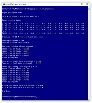
A good way to see where this article is headed is to take a look at the screenshot of a demo program, in Figure 1. The demo program creates a synthetic training dataset with 200 items. Each item has 10 input values and four output values. The first item's input values are (-0.8, 1.0, 6.8, -0.5, 0.1, 1.4, -5.0, 0.2, 2.1, 4.7). These are the predictor values, often called features in machine learning terminology. The four corresponding output values are: (0, 0, 1, 0).
The values-to-be-predicted (often called the labels) represent one of four categorical values. For example, the labels could represent the color of a car purchased and the features could represent normalized values such as buyer age, buyer income, buyer credit rating and so on. Suppose the four possible car color values are "red", ""white", "black" and "silver". Then (1, 0, 0, 0) represents "red"; (0, 1, 0, 0) is "white"; (0, 0, 1, 0) is "black"; and (0, 0, 0, 1) is "silver".
Behind the scenes, the demo also creates a 40-item set of test data that has the same characteristics as the 200-item training dataset.
The demo creates a 10-15-4 neural network classifier, that is, one with 10 input nodes, 15 hidden processing nodes and four output nodes. The number of input and output nodes is determined by the shape of the training data, but the number of hidden nodes is a free parameter and must be determined by trial and error.
Using back-propagation training without dropout, with 500 iterations and a learning rate set to 0.010, the network slowly improves (the mean squared error gradually becomes smaller during training). After training completes, the trained model has 98.00 percent classification accuracy on the training data (196 out of 200 correctly predicted). But the model achieves only 70.00 percent accuracy (28 out of 40 correct) on the previously unseen test data. It appears that the model may be overfitted.
Next, the demo resets the neural network and trains using dropout. After training, the model achieves 90.50 percent accuracy (181 out of 200 correct) on the test data, and 72.50 percent accuracy (29 out of 40 correct) on the test data. Although this is just a demonstration, this behavior is often representative of dropout training -- model accuracy on the test data is slightly worse, but accuracy on the test data, which is the metric that's most important, is slightly better.
 [Click on image for larger view.]
Figure 1. Neural Network Dropout Demo
[Click on image for larger view.]
Figure 1. Neural Network Dropout Demo
This article assumes you have a reasonably solid understanding of neural network concepts, including the feed-forward mechanism and the back-propagation algorithm, and that you have at least intermediate level programming skills. But I don't assume you know anything about dropout training. The demo is coded using Python version 3, but you should be able to refactor the code to other languages such as Python version 2 or C# without too much difficulty.
Program Structure
The demo program is too long to present in its entirety here, but the complete program is available in the accompanying download. The structure of the demo program, with a few minor edits to save space, is presented in Listing 1. Note that all normal error checking has been removed, and I indent with two space characters, rather than the usual four, to save space. The backslash character is used in Python for line continuation.
I used Notepad to edit the demo but most of my colleagues prefer one of the many nice Python editors that are available, including Visual Studio with the Python Tools for VS add-in. The demo begins by importing the numpy, random and math packages. Coding a neural network from scratch allows you to freely experiment with the code. The downside is the extra time and effort required.
Listing 1: Dropout Demo Program Structure
# nn_dropout.py
# Python 3.x

import numpy as np
import random
import math

# helper functions
def showVector(v, dec): . .
def showMatrix(m, dec): . .
def showMatrixPartial(m, numRows, dec, indices): . .
def makeData(genNN, numRows, inputsSeed): . .

class NeuralNetwork: . .

def main():
  print("Begin NN dropout demo ")

  print("Generating dummy training and test data \n")
  genNN = NeuralNetwork(10, 15, 4, 0)
  genNumWts = NeuralNetwork.totalWeights(10,15,4)

  genWeights = np.zeros(shape=[genNumWts], dtype=np.float32)
  genRnd = random.Random(3)
  genWtHi = 9.9; genWtLo = -9.9
  for i in range(genNumWts):
    genWeights[i] = (genWtHi - genWtLo) * \
      genRnd.random() + genWtLo
  genNN.setWeights(genWeights)

  dummyTrainData = makeData(genNN, numRows=200,
    inputsSeed=11)
  dummyTestData = makeData(genNN, 40, 13)
  print("Dummy training data: ")
  showMatrixPartial(dummyTrainData, 4, 1, True)

  numInput = 10
  numHidden = 15
  numOutput = 4
  print("Creating a %d-%d-%d neural network \
    classifier" % (numInput, numHidden, numOutput) )
  nn = NeuralNetwork(numInput, numHidden, numOutput,
    seed=2)

  maxEpochs = 500  # from 300, 500
  learnRate = 0.01
  print("Setting maxEpochs = " + str(maxEpochs))
  print("Setting learning rate = %0.3f " % learnRate)

  print("Starting training without dropout")
  nn.train(dummyTrainData, maxEpochs, learnRate,
    dropOut=False)
  print("Training complete")

  accTrain = nn.accuracy(dummyTrainData)
  accTest = nn.accuracy(dummyTestData)

  print("Accuracy on train data no dropout = \
    %0.4f " % accTrain)
  print("Accuracy on test data no dropout  = \
    %0.4f " % accTest)

  nn = NeuralNetwork(numInput, numHidden, numOutput,
    seed=2)
  dropProb = 0.50
  learnRate = 0.01
  print("Starting training with dropout ( %0.2f ) " \
    % dropProb)
  maxEpochs = 700  # need to train longer?
  nn.train(dummyTrainData, maxEpochs, learnRate,
    dropOut=True)
  print("Training complete")

  accTrain = nn.accuracy(dummyTrainData)
  accTest = nn.accuracy(dummyTestData)

  print("Accuracy on train data with dropout = \
    %0.4f " % accTrain)
  print("Accuracy on test data with dropout  = \
    %0.4f " % accTest)

  print("End demo ")

if __name__ == "__main__":
  main()
# end script
The demo program begins by generating the synthetic training and test data:
genNN = NeuralNetwork(10, 15, 4, 0)
genNumWts = NeuralNetwork.totalWeights(10,15,4)
genWeights = np.zeros(shape=[genNumWts], dtype=np.float32)
genRnd = random.Random(3)
genWtHi = 9.9; genWtLo = -9.9
for i in range(genNumWts):
  genWeights[i] = (genWtHi - genWtLo) * \
    genRnd.random() + genWtLo
genNN.setWeights(genWeights)
The approach used is to create a utility neural network with random, but known weight and bias values between -9.0 and +9.0, then feed the network random input values:
dummyTrainData = makeData(genNN, numRows=200,
  inputsSeed=11)
dummyTestData = makeData(genNN, 40, 13)
print("Dummy training data: \n")
showMatrixPartial(dummyTrainData, 4, 1, True)
Notice that the same utility neural network is used to generate both training and test data, but that the random input values are different, as indicated by the inputSeed parameter values of 11 and 13. Those seed values were selected only because they gave a representative demo.
Next, the neural network classifier is created:
numInput = 10
numHidden = 15
numOutput = 4
print("Creating a %d-%d-%d neural network \
  classifier" % (numInput, numHidden, numOutput) )
nn = NeuralNetwork(numInput, numHidden, numOutput, seed=2)
I cheated a bit by specifying 15 hidden nodes, the same number used by the data-generating neural network. This makes training easier. The seed value passed to the neural network constructor controls the random part of the dropout process and the order in which training item are processed. The value specified, 2, is arbitrary.
Next, the network is trained without using dropout:
maxEpochs = 500
learnRate = 0.01
nn.train(dummyTrainData, maxEpochs, learnRate, dropOut=False)
print("Training complete")
The NeuralNetwork class exposes dropout training via a parameter to the train method. Dropout is used here with standard back-propagation, but dropout can be applied to all training algorithms that use some form of gradient descent, such as back-propagation with momentum, back-propagation with regularization and the Adam and Nesterov algorithms.
After training completes, the accuracy of the model is computed and displayed:
accTrain = nn.accuracy(dummyTrainData)
accTest = nn.accuracy(dummyTestData)
print("Acc on train data no dropout =  %0.4f " % accTrain)
print("Acc on test data no dropout  =  %0.4f " % accTest)
The classification accuracy of the model on the test data is the more important of the two metrics. It gives you a very rough estimate of prediction accuracy of the model when presented new data, which is the ultimate goal of a classifier.
Next, the neural network is reset and trained, this time using dropout:
nn = NeuralNetwork(numInput, numHidden, numOutput, seed=2)
dropProb = 0.50
learnRate = 0.01
maxEpochs = 700
nn.train(dummyTrainData, maxEpochs, learnRate, dropOut=True)
print("Training complete")
Notice that with dropout, the maximum number of training iterations is increased from 500 to 700. In general, when using dropout, training will be slower and require more iterations than training without dropout.
The demo concludes by computing and displaying the classification accuracy of the dropout-trained model:
accTrain = nn.accuracy(dummyTrainData)
accTest = nn.accuracy(dummyTestData)
print("Acc on train data with dropout = %0.4f " % accTrain)
print("Acc on test data with dropout  = %0.4f " % accTest)
print("End demo ")
In this demo, using dropout slightly improved the classification accuracy on test data. However, even though using dropout often helps, in some problem scenarios using dropout can actually yield a worse model.
Understanding Dropout
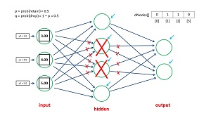
The dropout mechanism is illustrated in the diagram in Figure 2. The neural network has three input nodes, four hidden nodes and two output nodes and so does not correspond to the demo program. In back-propagation, on each training iteration, each node-to-node weight (indicated by the blue arrows) and each node bias (indicated by the green arrows) are updated slightly.
With dropout, on each training iteration, half of the hidden node are randomly selected to be dropped. Then the drop nodes essentially don't exist, so they don't take part in the computation of output node values, or in the computation of the weight and bias updates. In the diagram, if hidden nodes are 0-indexed, then hidden nodes [1] and [2] are selected as drop nodes on this training iteration.
Drop nodes aren't physically removed, instead they are virtually removed by having any code that references them ignored. In this case, in addition to hidden nodes [1] and [2], the six input-to-hidden weights that terminate in the drop nodes are ignored. And the four hidden-to-output node weights that originate from the drop nodes are ignored.
 [Click on image for larger view.]
Figure 2. The Neural Network Dropout Mechanism
[Click on image for larger view.]
Figure 2. The Neural Network Dropout Mechanism
What Figure 2 does not show is that after training, each input-to-hidden node weight, and each hidden-to-output node weight is divided by 2.0 (or equivalently, multiplied by 0.50). The idea here is that during training, there are effectively only half as many weights as there are in the final neural network. So during training, each weight value will be, on average twice as large as they should be. Dividing by 2.0 approximately restores the correct magnitudes of the weights for the full network. The exact math behind this idea is quite subtle and outside the scope of this article.
It's probably not obvious to you why dropout reduces overfitting. In fact, the effectiveness of dropout is not fully understood. One notion is that dropout essentially selects random subsets of neural networks, and then averages them together, giving a more robust final result. Another notion is that dropping hidden nodes helps prevent adjacent nodes from co-adapting with each other, again leading to a more robust model.
Implementation Issues
There are several approaches to implementing neural network dropout. The demo selects random nodes and then just ignores all occurrences of those nodes. For example, at the top of the training iteration loop, the demo code selects drop nodes like this:
if dropOut == True:
  for j in range(self.nh): # each hidden node
    p = self.rnd.random()  # [0.0, 1.0)
    if p < 0.50:
      self.dNodes[j] = 1  # mark as drop node
     else:
       self.dNodes[j] = 0  # not a drop node
The code checks the value of the Boolean dropOut parameter, then marks each hidden node as a dropout node or not, with probability equal to 0.50. Notice that using this approach, even though on average half of the hidden nodes will be selected as drop nodes, it's possible that on one iteration no nodes will be selected, or that all nodes will be selected. An alternative design that I have never seen used is to mark drop nodes in a way so that exactly half are selected each iteration.
When implementing class methods train and computeOutputs, the demo examines every reference to a hidden node and then checks if the node is currently a drop node or not. If the node is a drop node, it is skipped, otherwise the node is processed as usual. For example, in method computeOutputs, the part of the code that computes the pre-activation sum of products of the output nodes is:
for k in range(self.no): # each output node
  for j in range(self.nh): # each hidden node
    if dropOut == True and self.dNodes[j] == 1: # skip?
      continue
    oSums[k] += self.hNodes[j] * self.hoWeights[j,k]
  oSums[k] += self.oBiases[k]
An alternative approach, which I've seen used in several machine learning libraries, is instead of skipping over drop nodes, to set their values to 0.0. Then on the forward pass through the network, all the key terms zero-out. However you still must skip over drop nodes on the backwards pass during training.
Wrapping Up
There are several types of dropout. In addition to dropping hidden nodes, it's possible to drop input nodes. And instead of randomly dropping nodes with probability equal to 0.50, you can drop fewer or more nodes. For example, you can drop with probability equal to 0.20, or drop with probability equal to 0.80. If so, you have to be careful to modify the final network weight values accordingly. Suppose you drop nodes with probability equal to 1/5 = 0.20. That means on average the training network has 80 percent of the weights of the full network, in other words the trained weights will be slightly too large. So, you'd multiply all weights by 0.80 (or equivalently, divide by 1.25) to reduce their magnitudes slightly.
There are several techniques, other than dropout, that you can use to combat neural network overfitting. Common techniques include:
If you're new to neural networks, all these options can seem a bit overwhelming, but if you explore them one at a time, eventually the larger picture becomes clear.