The Data Science Lab
Decision Tree Regression from Scratch Using JavaScript
Dr. James McCaffrey presents a complete end-to-end demonstration of decision tree regression from scratch using JavaScript. The goal of decision tree regression is to predict a single numeric value. For simplicity and better maintenance, the demo implementation uses list storage instead of pointers. For better customization and interpretability, the implementation uses list iteration instead of recursion or a stack algorithm.
Decision tree regression is a machine learning technique that incorporates a set of if-then rules in a tree data structure to predict a single numeric value. For example, a decision tree regression model prediction might be, "If employee age is greater than 28.0 and age is less than or equal to 32.5 and years-experience is less than or equal to 5.0 and height is greater than 66.0 then bank account balance is $833.127."
There are many ways to implement a decision tree regression system. Four significant design decisions are 1.) use pointers/references for tree nodes, or use list storage, 2.) use recursion to construct the tree, or use a non-recursive stack, or use list iteration, 3.) use weighted variance minimization for the node split function, or use variance reduction maximization, 4.) explicitly store row indices associated with each node in the nodes, or discard the associated rows information after use during training. There are pros and cons to each option.
This article presents decision tree regression, implemented from scratch with JavaScript, using list storage for tree nodes (no pointers/references), list iteration to build the tree (no recursion or stack), weighted variance minimization for the node split function, and saves associated row indices in each node. This design has maximum flexibility.
A single decision tree can be used by itself for regression problems. But a more common approach is to use a collection of decision trees, called an ensemble technique. Examples include bagging tree regression, random forest regression, adaptive boosting regression, and gradient boosting regression. The decision tree design presented in this article can be easily adapted for any ensemble technique. But regardless of which tree technique is used, everything starts with a decision tree.
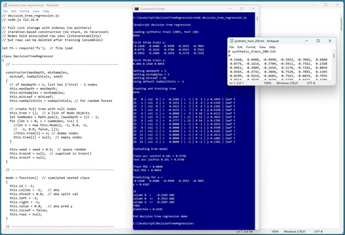
A good way to see where this article is headed is to take a look at the screenshot in Figure 1 and the related diagram in Figure 2. The demo program begins by loading synthetic training and test data into memory. The data looks like:
-0.1660,  0.4406, -0.9998, -0.3953, -0.7065,  0.4840
 0.0776, -0.1616,  0.3704, -0.5911,  0.7562,  0.1568
-0.9452,  0.3409, -0.1654,  0.1174, -0.7192,  0.8054
 0.9365, -0.3732,  0.3846,  0.7528,  0.7892,  0.1345
. . .
The first five values on each line are the x predictors. The last value on each line is the target y variable to predict. The demo creates a decision tree model, evaluates the model accuracy on the training and test data, and then uses the model to predict the target y value for x = [-0.1660, 0.4406, -0.9998, -0.3953, -0.7065].
 [Click on image for larger view.] Figure 1
: Decision Tree Regression in Action Using JavaScript.
[Click on image for larger view.] Figure 1
: Decision Tree Regression in Action Using JavaScript.
The first part of the demo output shows how a decision tree is created:
Loading synthetic train (200) and test (40) data
Done

Setting maxDepth = 3
Setting minSamples = 2
Setting minLeaf = 18
Using default numSplitCols = -1
Creating and training tree
Done
A decision tree regression system has four parameters that control the size, shape, and behavior of the tree: maxDepth, minSamples, minLeaf, numSplitCols. Briefly, maxDepth sets a maximum number of levels, and minSamples and minLeaf set node splitting granularity. The numSplitCols parameter is a regularization technique that is used when a decision tree is part of a random forest regression model.
For the demo, maxDepth is set to an artificially small value (3) and minLeaf is set to an artificially large value (18) to create a small tree that can be easily visualized. The demo uses a special -1 value for numSplitCols that means "use all columns when computing splits."
The next part of the demo output displays the trained decision tree:
ID   0 | col  0 | v  -0.2102 | L  1 | R  2 | y 0.3493 | leaf F
ID   1 | col  4 | v   0.1431 | L  3 | R  4 | y 0.5345 | leaf F
ID   2 | col  0 | v   0.3915 | L  5 | R  6 | y 0.2382 | leaf F
ID   3 | col  4 | v  -0.4391 | L  7 | R  8 | y 0.6358 | leaf F
ID   4 | col -1 | v   0.0000 | L  9 | R 10 | y 0.4123 | leaf T
ID   5 | col  4 | v  -0.2987 | L 11 | R 12 | y 0.3032 | leaf F
ID   6 | col  1 | v   0.0863 | L 13 | R 14 | y 0.1701 | leaf F
ID   7 | col -1 | v   0.0000 | L -1 | R -1 | y 0.6895 | leaf T
ID   8 | col -1 | v   0.0000 | L -1 | R -1 | y 0.5793 | leaf T
ID  11 | col -1 | v   0.0000 | L -1 | R -1 | y 0.4101 | leaf T
ID  12 | col -1 | v   0.0000 | L -1 | R -1 | y 0.2613 | leaf T
ID  13 | col -1 | v   0.0000 | L -1 | R -1 | y 0.1503 | leaf T
ID  14 | col -1 | v   0.0000 | L -1 | R -1 | y 0.1986 | leaf T
Each row is a tree node. The fields are node ID, index of split column (or -1 if the node cannot be split because it's a leaf node), split threshold value (or 0.0000 if the node cannot be split), (L)eft child index, (R)ight child index, predicted y value, and a Boolean indicating if the node is a leaf node (T)rue or not (F)alse). The tree is shown as a diagram in Figure 2.
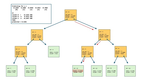 [Click on image for larger view.] Figure 2: Visual Representation of the Demo Decision Tree Regression Model.
Notice that tree nodes [9] and [10] are empty nodes, so they are not displayed in Figure 1 or Figure 2.
The next part of the demo output shows the tree model evaluation metrics:
Evaluating model
Accuracy train (within 0.10) = 0.3750
Accuracy test (within 0.10) = 0.4750
MSE train = 0.0048
MSE test = 0.0054
The accuracy of the prediction model is poor. The model scores just 37.50% (75 correct out of 200) on the training data and 47.50% (19 out of 40) on the test data. A prediction is scored as correct if it's within 10% of the true target y value. The accuracy and MSE (mean squared error) are weak because maxDepth is too small and minLeaf is too large (to keep the tree small enough for easy visualization). By setting maxDepth = 7, minSamples = 2, minLeaf = 1, numSplitCols = -1, the decision tree scores 91.00% accuracy on the training data.
The last part of the demo output shows an example prediction:
Predicting for trainX[0] =
  -0.1660   0.4406  -0.9998  -0.3953  -0.7065
Predicted y = 0.4101

IF
column 0  >   -0.2102 AND
column 0  <=  0.3915 AND
column 4  <= -0.2987 AND
THEN
predicted = 0.4101
One advantage of decision tree regression compared to other techniques, such as kernel ridge regression and neural network regression, is that decision trees are significantly more interpretable. If you examine the diagram in Figure 2, and follow the red dashed arrows, you can see exactly how the predicted y value is computed.
This article assumes you have intermediate or better programming skill but doesn't assume you know anything about decision tree regression. The demo is implemented using JavaScript, but you should be able to refactor the demo code to a C-family language if you wish. All normal error checking has been removed to keep the main ideas as clear as possible.
The source code for the demo program is too long to be presented in its entirety in this article. The complete code and data are available in the accompanying file download, and they're also available online.
The Demo Data
The demo data is synthetic. It was generated by a 5-10-1 neural network with random weights and bias values. The idea here is that the synthetic data does have an underlying, but complex, structure which can be predicted.
All of the predictor values are between -1 and +1. There are 200 training data items and 40 test items. When using decision tree regression, it's not necessary to normalize the training data predictor values because no distance between data items is computed. However, normalizing the predictors doesn't hurt and it's useful just in case you want to send the data to another regression algorithm that requires normalization, for example, nearest neighbors regression or kernel ridge regression.
In practice, decision tree regression is most often used with data that has strictly numeric predictor variables. But it is possible to use decision tree regression with categorical data. For ordinal categorical data that has inherent ordering, you can use standard zero-based or one-based ordinal encoding. For example, for a predictor variable employee-height with possible values (short, medium, tall), you could set short = 0, medium = 1, tall = 2.
For binary data, you can use zero-one encoding. For example, for a predictor variable employee-sex, you could set male = 0, female = 1, or vice versa.
For nominal categorical data without inherent order, in theory, decision tree regression isn't applicable. But in practice, standard zero-based or one-based ordinal encoding often works quite well. For example, suppose you have a predictor variable citizenship with possible values (Australia, Canada, Germany, Japan, Sweden). You could set Australia = 0, Canada = 1, Germany = 2, Japan = 3, Sweden = 4. One internal node of the decision tree might be, "If column [7] <=2 Then go left." This would group Australia, Canada, Germany together, and Japan, Sweden together.
The downside of ordinal encoding nominal categorical data is that the resulting tree has a significant dependency on the order in which you encode the data. The upside is that if the tree is deep enough, the technique often works well.
Understanding Tree Storage Using a List
The demo decision tree has maxDepth = 3. This creates a tree with 15 nodes (some of which could be empty). In general, if a tree has maxDepth = n, then it has 2^(n+1) - 1 nodes. These tree nodes could be stored as separate program-defined Node objects that are connected via pointers/references. But the architecture used by the demo decision tree is to create a JavaScript list collection with size/length = 15, where each item in the list is a Node object.
With this design, if the root node is at index [0], then the left child is at [1] and the right child is at [2]. In general, if a node is at index [i], then the left child is at index [2*i+1] and the right child is at index [2*i+2]. This design also allows you to easily save a decision tree to file storage.
If a node is empty, there is very little memory space wasted because node objects are references that can be set to null.
Understanding Decision Tree Regression - Splitting
The tree splitting part of constructing a decision tree regression system is best understood by looking at a concrete example. The root node of the demo decision tree is associated with all 200 rows of the training data. The splitting process selects some of the 200 rows to be assigned to the left child node, and the remaining rows to be assigned to the right child node.
For simplicity, suppose that instead of the demo training data with 200 rows and 5 columns of predictors, a tree node is associated with just five rows of data, and the data has just three columns of predictors:
     X                    y
[0] 0.97  0.25  0.75     3.0
[1] 0.53  0.41  0.00     9.0
[2] 0.86  0.64  0.86     7.0
[3] 0.14  0.37  0.25     2.0
[4] 0.53  0.86  0.37     6.0
     [0]   [1]   [2]
The split algorithm will select some of the five rows to go to the left child and the remaining rows to go to the right child. The idea is to select the two sets of rows in a way so that their associated y values are close together. The demo implementation does this by finding the split that minimizes the weighted variance of the target y values.
The splitting algorithm examines every possible x value in every row and every column. For each possible candidate split value (also called the threshold), the weighted variance of the y values of the resulting split is computed. For example, for x = 0.37 in column [1], the rows where the values in column [1] are less than or equal to 0.37 are rows [3] and [0] with associated y values (2.0, 3.0). The other rows are [1], [2], [4] with associated y values (9.0, 7.0, 6.0).
The variance of a set of y values is the average of the sum of the squared differences between the values and their mean (average).
For this proposed split, the variance of y values (2.0, 3.0) is computed as 0.25. The mean of (2.0, 3.0) = (2.0 + 3.0) / 2 = 2.5 and so the variance is ((2.0 - 2.5)^2 + (3.0 - 2.5)^2) / 2 = 0.25.
The mean of y values (9.0, 7.0, 6.0) = (9.0 + 7.0 + 6.0) / 3 = 7.33 and the variance is ((9.0 - 7.33)^2 + (7.0 -7.33)^2 + (6.0 - 7.33)^2) / 3 = 2.33.
Because the proposed split has different numbers of rows (two rows for the left child and three rows for the right child), the weighted variance of the proposed split is used and is ((2 * 0.25) + (3 * 2.33)) / 5 = 1.50.
This process is repeated for every x value in the training data. The x threshold value and its column that generate the smallest weighted variance define the split. In practice it's common to keep track of which values in a given column have already been checked, to avoid unnecessary work computing weighted variance.
After a best split is found, the predicted y value for a leaf node (no further splits) is the average of the y values associated with the node. The demo program computes predicted y values for internal, non-leaf nodes, but those predicted values are not used except when debugging.
A source of minor vocabulary confusion is that the term "mean squared error" can have two different meanings in machine learning. In most scenarios, mean squared error is used to evaluate how well a model predicted values match the known correct target values in the training data. This standard MSE is the average of the squared differences between predicted y values and correct target y values.
But in some decision tree regression splitting contexts, notably the scikit-learn Python library, sometimes mean squared error is used as a synonym for variance. The idea is that in a decision tree, the predicted values are the y values of a split and the virtual correct target y values are all identical, the mean of the y values.
Implementing the Split Function
When implementing a decision tree split function, the minSamples parameter specifies the minimum number of rows associated with a node necessary before a split is to be considered. In practice this is usually set to 2 which leads to many splits and a more granular tree.
The minLeaf parameter specifies the minimum number of rows required after a split is performed. In practice this is usually set to 1 which allows leaf nodes with a single associated y value, but prohibits any leaf nodes with no associated y values, which is logically inconsistent.
A common decision tree technique is to randomly shuffle the order in which columns are examined when looking for the best split. The idea here is that without shuffling, the first predictor columns have priority over later columns in cases where there are multiple split values that produce the same minimum mean squared error. Shuffling the order of columns prevents a bias towards early columns, but introduces a small amount of randomness into a decision tree regression system.
The numSplitCols parameter specifies how many of the columns of the X data should be examined when looking for a split value and split column. In almost all scenarios, you want to examine all columns. An exception is when a collection of decision trees is used for a random forest regression system where there are many predictor variables. The DecisionTreeRegressor has a default value of -1 for numSplitCols, which is a special value that means to "use all columns."
Understanding Decision Tree Regression - Building
There are three main approaches for building a regression decision tree: using recursion, or using a stack data structure, or using list iteration. The most common technique presented in online examples is to use recursion. I suspect this is mostly because building a decision tree using recursion is elegant and fancy. However, many of the software production teams that I have worked with have a formal ban on the use of any kind of recursion in production code. Recursive code is tricky to implement, tricky to debug, tricky to profile, and tricky to modify.
The demo program uses list iteration to construct the decision tree. In high-level pseudo-code:
create a list of empty/null tree nodes
create root node at index [0]
for-each node in list
  get curr node
  if curr node too deep to have children OR not enough rows to split then
    node is a leaf, predicted = avg of associated Y values
  compute split value and split column rows in curr node
  if unable to split then
    node is a leaf, predicted = avg of associated Y values
  compute left-rows, right-rows, left node, right node
  add left node to list; add right node to list
end-for
The build-tree algorithm is short but very tricky. Storing the rows that are associated with a node is a design that allows you to diagnose how the tree was constructed. If for some reason you want to minimize memory usage for huge decision trees, you can add code to the end of the train() method to remove the stored rows in all nodes, because they're not needed after training.
The Demo Program
I used old-fashioned Notepad to edit the demo program. You will mostly likely want to use a more sophisticated editor. Visual Studio Code is a popular choice among my work colleagues.
The demo program was written for a node.js environment. The demo program was developed using version v22.16.0 but any relatively recent version will work.
The overall program structure is presented in Listing 1. All the control logic is in a main() function. All of the decision tree regression functionality is in a DecisionTreeRegressor class. The DecisionTreeRegressor class exposes a constructor and six core methods: train(), predict(), explain(), accuracy(), mse(), and display(). The class has seven helper methods, and there are two helper function for the main() function.
Listing 1: Overall Program Structure
// decision_tree_regression.js
// node.js v22.16.0

let FS = require('fs');  // file load

class DecisionTreeRegressor
{
  // --------------------------------------------------------

  constructor(maxDepth, minSamples,
    minLeaf, numSplitCols, seed) { . . }

  // --------------------------------------------

    Node = function() { . . }

  // --------------------------------------------

  // core methods
  train(trainX, trainY) { . . }
  predict(x) { . . }
  explain(x) { . . }
  accuracy(dataX, dataY, pctClose) { . . }
  mse(dataX, dataY)
  display(showRows)

  // helpers for train()
  makeTree() { . . }
  bestSplit(rows) { . . }
  next() { . . }
  nextInt(lo, hi) { . . }
  shuffle(indices) { . . }
  treeTargetMean(rows) { . . }
  treeTargetVariance(rows) { . . }

} // DecisionTreeRegressor

// helpers for main()
function loadTxt(fn, delimit, usecols, comment) { . . }
function vecShow(v, dec, len) { . . }

// ----------------------------------------------------------

function main()
{
  console.log("JavaScript decision tree regression ");

  // 1. load data
  // 2. create and train tree
  // 3. evaluate tree
  // 4. use tree to make prediction

  console.log("End decision tree regression demo ");
}

main();
The explain() method is essentially a verbose version of the predict() method. The makeTree() helper does most of the work for the train() method.
Because JavaScript does not support nested classes, the DecisionTreeRegressor class uses relatively rare (to me anyway) syntax to simulate a Node container class. The idea is to keep the code as self-contained as possible.
Loading the Training and Test Data
The demo starts by loading the 200-item training data and 40-item test data into memory:
let trainFile = ".\\Data\\synthetic_train_200.txt";
let trainFile = ".\\Data\\synthetic_train_200.txt";
let testFile = ".\\Data\\synthetic_test_40.txt";

let trainX = loadTxt(trainFile, ",", [0,1,2,3,4], "#");
let trainY = loadTxt(trainFile, ",", [5], "#");
let testX = loadTxt(testFile, ",", [0,1,2,3,4], "#");
testY = loadTxt(testFile, ",", [5], "#");
The training X data is stored into an array-of-arrays style matrix. The data is assumed to be in a directory named Data, which is located in the project root directory. The arguments to the loadTxt() function for trainX mean load columns 0, 1, 2, 3, 4 where the data is comma-delimited, and lines beginning with "#" are comments to be ignored. The training y data in column [5] is loaded into a matrix and then converted to a one-dimensional vector behind the scenes. I use the somewhat strange "loadTxt" name because the demo function is inspired by the NumPy loadtxt() library function.
Next, the first three training items are displayed using these statements:
console.log("First three train x: ");
for (let i = 0; i < 3; ++i)
  vecShow(trainX[i], 4, 8);  // 4 decimals 8 wide
console.log("First three train y: ");
for (let i = 0; i < 3; ++i)
  process.stdout.write(trainY[i].toString() + " ");
console.log("");
In a non-demo scenario, you might want to display all the training data to make sure it was correctly loaded into memory.
Training the Decision Tree
The decision tree regression model is trained/fit/constructed like so:
let maxDepth = 3;
let minSamples = 2;
let minLeaf = 18;
let numSplitCols = -1;  // all columns
let seed = 0;

let dtr =
  new DecisionTreeRegressor(maxDepth, minSamples,
    minLeaf, numSplitCols, seed);
dtr.train(trainX, trainY);
dtr.display(false); // show rows or not
If maxDepth is set to 0, the tree has just a single (root) node and the predicted y value for any input is the average of the training y data. If maxDepth is set to 1, the tree has at most three nodes: root node, left child, right child. If maxDepth is set to 2, the tree has at most seven nodes. In general, if maxDepth is set to n, the tree has at most 2^(n+1) - 1 nodes.
Decision trees are often sensitive to pathological data, and it's usually a good idea to display a trained tree to look for various abnormalities.
Each tree node holds the indices of the rows of training data. When the showRows parameter is set to false, the associated rows are not displayed. If showRows is set to true, the output would resemble:
ID   0 | col  0 | v  -0.2102 | L  1 | R  2 | y 0.3493 | leaf F
rows: 0  1  2  3  4 . . 198  199

ID   1 | col  4 | v   0.1431 | L  3 | R  4 | y 0.5345 | leaf F
rows: 2  4  6  8  9 . . 198  199

ID   2 | col  0 | v   0.3915 | L  5 | R  6 | y 0.2382 | leaf F
rows: 0  1  3  5  7 . . 195  197
. . .
The root node with ID = 0 is associated with all 200 of the rows of the training data. The left child with ID = 1 is associated with about half of all the rows, and the right child with ID = 2 is associated with the remaining rows.
Evaluating and Using the Decision Tree
Next, the demo evaluates model accuracy:
let trainAcc = dtr.accuracy(trainX, trainY, 0.10);
let testAcc = dtr.accuracy(testX, testY, 0.10);
console.log("Train acc (within 0.10) = " + trainAcc.toFixed(4).toString());
console.log("Test acc (within 0.10) = " + testAcc.toFixed(4).toString());
The Accuracy() method scores a prediction as correct if it's within 10% of the true target y value. The 10% is arbitrary and a reasonable closeness percentage will vary from problem to problem.
The demo computes model mean squared error using these statements:
let trainMSE = dtr.mse(trainX, trainY);
let testMSE = dtr.mse(testX, testY);
console.log("Train MSE = " + trainMSE.toFixed(4).toString());
console.log("Test MSE = " + testMSE.toFixed(4).toString());
In addition to accuracy and MSE, another common model evaluation metric is the coefficient of determination, R2. See this article for details.
The demo concludes by using the trained decision tree to make a prediction in two ways:
let x = trainX[0];
console.log("Predicting for x = ");
vecShow(x, 4, 9);
let predY = dtr.predict(x);
console.log("y = " + predY.toFixed(4).toString());
dtr.explain(x);
The predict() method spits out the predicted y value without any explanation. The explain() method is essentially a verbose predict function.
Wrapping Up
Implementing decision tree regression from scratch requires a significant amount of effort, but it allows you to easily integrate a prediction model with other web-based systems. A from-scratch implementation also allows you to easily modify the system. For example, you can comment-out the code statements that shuffle the order in which columns are processed in the split function, so that your decision tree is completely deterministic. Or you can add only error-checking that's relevant for your scenario.
The biggest disadvantage of a simple decision tree regression system is that a single tree usually overfits the training data. In overfitting, the trained model predicts well on the training data, but predicts poorly on new, previously unseen data. Because of the overfitting problem, decision trees are rarely used by themselves. Instead, multiple trees are combined into an ensemble model such as bagging tree regression, random forest regression, adaptive boosting regression, or gradient boosting regression. The decision tree design presented in this article is well-suited for use in ensemble models.